Excel 2013 -
Tables

Excel 2013
Tables


search
menu
/en/excel2013/groups-and-subtotals/content/
Once you've entered information into a worksheet, you may want to format your data as a table. Just like regular formatting, tables can improve the look and feel of your workbook, but they'll also help to organize your content and make your data easier to use. Excel includes several tools and predefined table styles, allowing you to create tables quickly and easily.
Optional: Download our practice workbook.
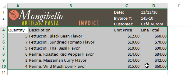 Selecting a cell range to format as a table
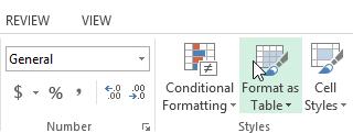 Clicking the Format as Table command
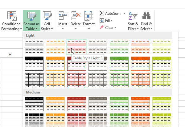 Choosing a table style
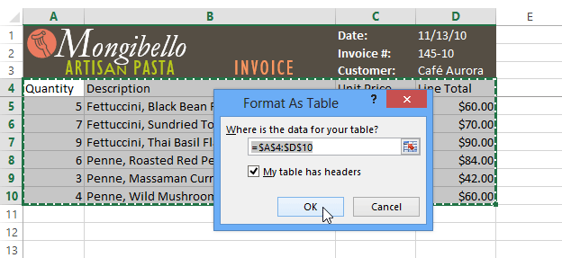 Clicking OK
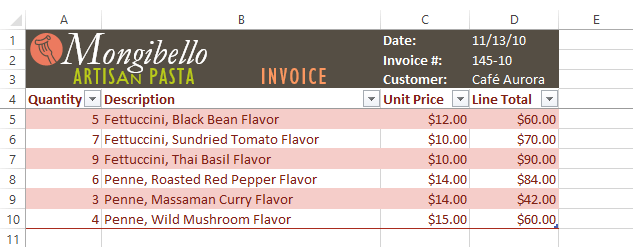 The cell range formatted as a table
Tables include filtering by default. You can filter your data at any time using the drop-down arrows in the header cells. To learn more, review our lesson on Filtering Data.
It's easy to modify the look and feel of any table after adding it to a worksheet. Excel includes different options for customizing a table, including adding rows or columns and changing the table style.
If you need to fit more content in your table, Excel allows you to modify the table size by including additional rows and columns. There are two simple ways to change the table size:
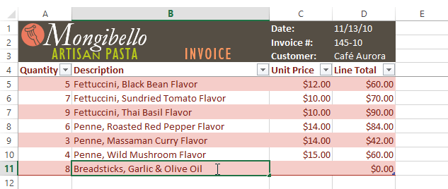 Typing a new row below an existing table
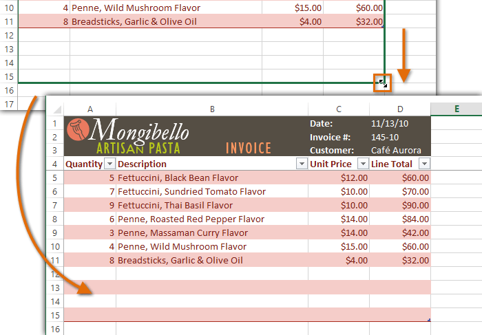 Dragging the table border to create more rows
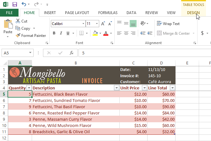 Clicking the Design tab
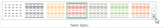 Clicking the More drop-down arrow
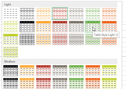 Choosing a new table style
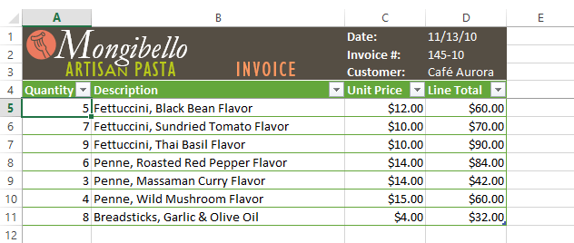 The new table style
You can turn various options on or off to change the appearance of any table. There are several options: Header Row, Total Row, Banded Rows, First Column, Last Column, Banded Columns, and Filter Button.
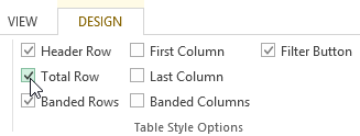 Checking the Total Row option
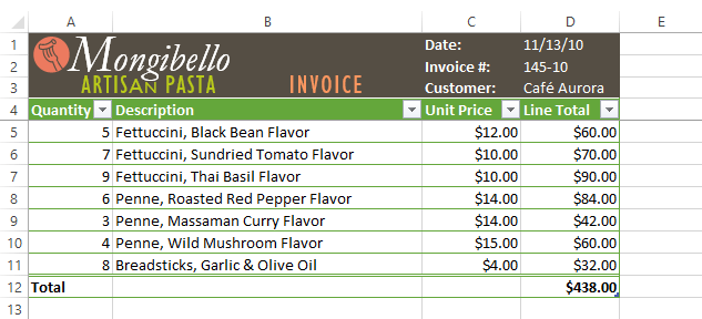 The table with a total row
These options can affect your table style in various ways, depending on the type of content in your table. You may need to experiment with a few different options to find the exact style you want.
Sometimes you may not want to use the additional features included with tables, such as the Sort and Filter drop-down arrows. You can remove a table from the workbook while still preserving the table's formatting elements, like font and cell color.
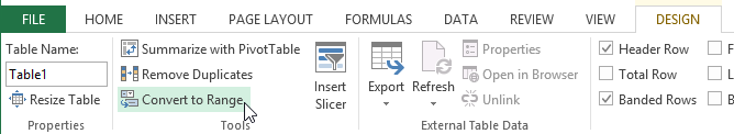 Clicking Convert to Range
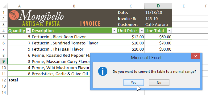 Removing a table
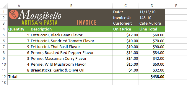 The cell range formatted as a normal range
/en/excel2013/charts/content/