Lesson 22: Invoice, Part 3: Fix Broken VLOOKUP
/en/excelformulas/invoice-part-2-using-vlookup/content/

"Hey, it's me again…so, I think I might have broken that VLOOKUP formula you created.
I put a few new products into the Products worksheet, but the VLOOKUP function is having trouble pulling in the new data. Could you take a look and see if you can fix it?"
This lesson is part 3 of 5 in a series. You can go to Invoice, Part 1: Free Shipping if you'd like to start from the beginning.
Our spreadsheet
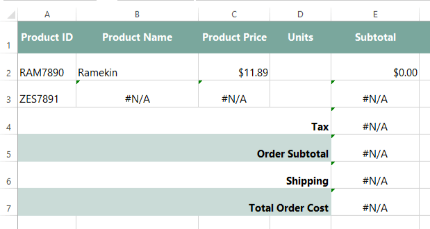
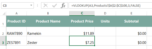
Once you've downloaded our spreadsheet, open the file in Excel or another spreadsheet application. The VLOOKUP function in row 2 looks good, but row 3 doesn't seem to be working. And since the formulas in column E depend on the values in row 3, they're not able to calculate correctly.
What are we trying to fix?
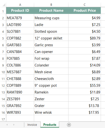
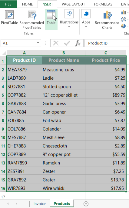
Let's see if we can figure out what went wrong. Our coworker added some new products to the Products worksheet, but they don't work with the existing VLOOKUP functions. If we look at the Products worksheet, we can see that there are a few new products listed here. The data spans cell range A2:C16.
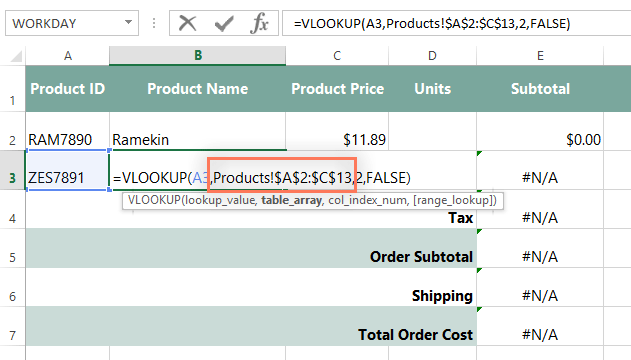
But if we look at the function in cell B3, we can see that the VLOOKUP function is only searching for information in cell range A2:C13.
As you can see, the VLOOKUP function isn't searching the full list of products; it's only searching down to row 13. So it has no trouble finding the Ramekin, but it won't be able to find the Zester, Grater, or Wire whisk.
To fix this, we'll need to change the second argument in VLOOKUP so it searches the entire product list. There are two ways to do this:
- Update the cell ranges
- Use a table (Microsoft Excel only)
Update the cell ranges
One way to fix this problem is to simply update the cell ranges in our VLOOKUP functions. Let's try editing the function in cell B3, where it's stopped working.
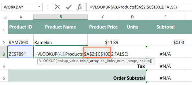
We'll edit the function to include all of the cells in the Products table. And just in case more products are added later, we'll increase the number of rows in the cell range to 100. This means we're including a lot of empty rows, but that's OK—the VLOOKUP function will still work the same way. So here's our new function:
=VLOOKUP(A3, Products!$A$2:$C$100, 2, FALSE)
The function will recalculate, and the correct product name should appear: Zester. We'll also make the same correction to the remaining VLOOKUP functions in the spreadsheet:
And that's it! Now our spreadsheet's working correctly, and it'll be harder to break these functions in the future.
Use a table
Above, we fixed our VLOOKUP function by extending the cell range to row 100. However, if we continue adding more products, we will eventually break the VLOOKUP function again, so this is not a perfect solution. If you're using Microsoft Excel, a much better solution is to use a table. This will ensure that any new data will be included automatically.
Tables work with all recent versions of Excel, but they are not currently available in Google Sheets.
First, we'll select our product information and then convert it to a table. Note that this will work a bit differently depending on which version of Excel you're using:
- For Excel 2007-2019: Go to Insert > Table.
- For Excel 2003 and earlier: Go to Data > List > Create List (tables were known as lists in Excel 2003 and earlier).
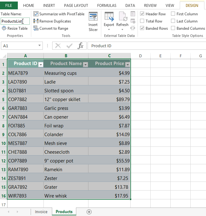
Next, we'll name the table. In this example, we'll give it the name: ProductsList. Note that table names cannot contain spaces.
Now let's go back to our VLOOKUP function. Rather than telling VLOOKUP to search in a specific range on the Products worksheet (Products!$A$2:$C$100), we can simply type the name of the table (ProductsList).
So here's our new function:
=VLOOKUP(A3, ProductsList, 2, FALSE)
If anyone ever adds information to the table, the VLOOKUP function will include it automatically—no need to worry about updating the cell range later on. Again, you'll need to update all of the VLOOKUP functions in the spreadsheet to refer to the table rather than the cell range.

"It's working again? Fantastico!
I guess I should have realized that adding more products could break the formula, but I'm glad that won't be an issue in the future. Thanks!"
If you'd like to continue on to the next part in this series, go to Invoice, Part 4: More Shipping Options.
/en/excelformulas/invoice-part-4-more-shipping-options/content/