Excel 2003: Creating Complex Formulas

Lesson 6: Creating Complex Formulas

/en/excel2003/creating-simple-formulas/content/

Introduction

By the end of this lesson, you should be able to:

Create complex formulas
Fill a formula to another cell
Copy and paste a formula into another cell
Revise a formula
Create an absolute reference

Complex formulas defined

Simple formulas have one mathematical operation. Complex formulas involve more than one mathematical operation.

The order of mathematical operations is important. If you enter a formula that contains several operations—like adding, subtracting, and dividing—Excel 2003 knows to work these operations in a specific order. The order of operations is:

Operations enclosed in parenthesis
Exponential calculations (to the power of)
Multiplication and division, whichever comes first
Addition and subtraction, whichever comes first

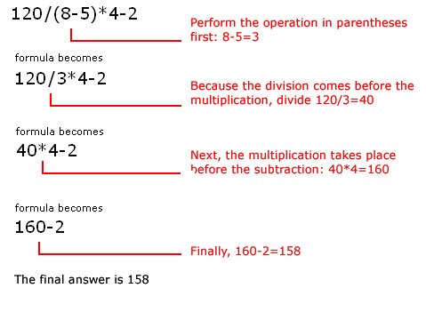
Using this order, let's see how the formula 120/(8-5)*4-2 is calculated in the following picture:

Breakdown of a Complex Formula

Let's take a look at another example:

2*(6-4) =?

Is the answer 8 or 4? If you ignored the parentheses and calculated in the order in which the numbers appear, 2*6-4, you'd get the wrong answer, 8. You must follow the order of operations to get the correct answer.

To calculate the correct answer:

Calculate the operation in parenthesis (6-4), where the answer is 2.
Multiply the answer obtained in step 1, which is 2, to the numeric 2* that opened the equation. In other words, multiply 2*2.
The answer is 4.

When using formulas with cell references, the results change each time the numbers are edited.

Remember: In Excel, never do math "in your head" and type the answer in a cell where you would expect to have a formula calculate the answer.

Complex formulas defined

Before moving on, let's explore some more formulas to make sure you understand the order of operations by which Excel calculates the answer.

*53/2**	Multiply 53 before performing the division operation because the multiplication sign comes before the division sign. The answer is 7.5*.
*5/32**	Divide 5/3 before performing the multiplication operation because the division sign comes before the multiplication sign. The answer is 3.333333.
*5/(32)**	Perform the operation in parentheses (32) first, and divide 5 by this result. The answer is 0.833333*.
5+3-2	Add 5+3 before performing the subtraction operation because the addition sign comes before the subtraction sign. The answer is 6.
5-2+3	Subtract 5-2 before performing the addition operation because the subtraction sign comes before the addition sign. The answer is 6.
*5-23**	Multiply 2*3 before performing the subtraction operation because the multiplication sign is of a higher order than the subtraction sign. The answer is -1.
*(5-2)3**	Perform the operation in parenthesis (5-2) first and then multiply by 3. The answer is 9.

Creating complex formulas

Excel 2003 automatically follows a standard order of operations in a complex formula. If you want a certain portion of the formula to be calculated first, put it in parentheses.

If we wanted to add the contents of cell B2 and cell B3, for example, and then take that answer and multiply it by the data in cell A4, we would need to define the following formula: =(B2+B3)*A4.

A Complex Formula

Enter the numbers you want to calculate.
Click the cell where you want the formula result to appear.
Type the equals sign (=) to let Excel know that a formula is being defined.
Type an open parenthesis, or (.
Click the first cell to be included in the formula (cell B2, for example).
Type the addition sign (+) to let Excel know that an add operation is to be performed.
Click the second cell in the formula. The reference B3 displays where you want your result.
End the B2+B3 operation by adding the close parenthesis, or ).
Type the next mathematical operator, or the multiplication symbol (*), to let Excel know that a multiply operation is to be performed.
Click the third cell to be included in the formula, cell A4.
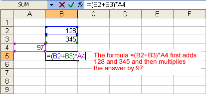
Press Enter, or click the Enter button on the Formula bar. This step ends the formula.

Try changing one of the values in the formula, then watch the answer to the formula change.

Excel will not always tell you if your formula contains an error, so it's up to you to check all of your formulas. To learn how to do this, you can read the Double-Check Your Formulas lesson from our Excel Formulas tutorial.

Filling formulas to other cells

Sometimes you will write a formula that gets used a lot in different places of a worksheet. For example, a spreadsheet may contain several columns of numbers. Each column will contain a formula that adds all of the numbers in it. You could write the formula several times, once in each column. Or you could copy and paste it into each column. The fill formula method allows you to copy a formula and then fill it into many different consecutive cells at the same time.

The mouse pointer changes to a black crosshair when passed over the fill handle, or the square box in the lower right corner of the cell.

The Fill Handle

To use the fill handle to copy a formula to a surrounding cell:

Click the cell that contains the formula to be copied.
Position the mouse pointer over the fill handle.
Click and hold the left mouse button, then drag the contents to the cell that will receive the fill formula.
Release the mouse button.
Select the Copy Cells option in the fill formula drop-down menu.

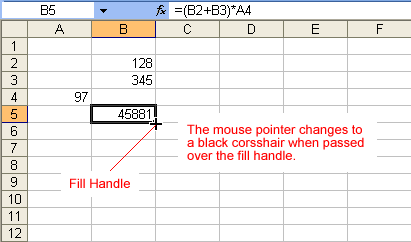
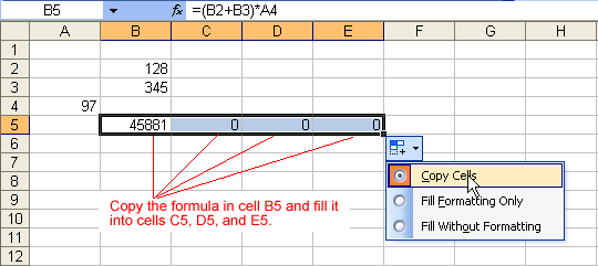
The cell references in a formula are automatically updated when the formula is copied to other cells in the spreadsheet.

You can also use copy and paste to copy a formula to other cells. Click next to learn more about the copy and paste method.

Copy and paste formulas

The process to copy and paste a formula is identical to that process used to copy and paste text.

To copy and paste a formula:

Select the cell that contains the formula to be copied.
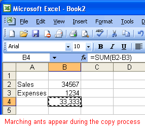
Click the Copy button. Marching "ants" appear around the copied cell(s).
Select the cell where the copied formula is to be pasted.
Press the Enter key. The formula is copied to the new location.

Revising formulas

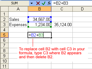
You can revise any formula that was previously written in a worksheet.

To revise a formula using the keyboard:

Double-click the cell that contains the formula you want to revise.
The cursor can now move left and right between the values in the formula in cell B5.
Make the necessary changes to the formula.
Press the Enter key, or click the Enter button to accept the new formula.

Creating an absolute reference

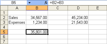
In earlier lessons, we saw how cell references in formulas automatically adjust to new locations when the formula is pasted into different cells.

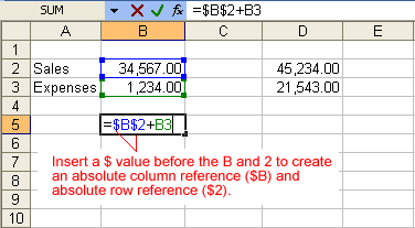
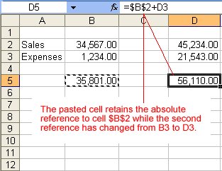
Sometimes when you copy and paste a formula, you don't want one or more cell references to change. An absolute reference solves this problem. Absolute cell references in a formula always refer to the same cell or cell range in a formula. If a formula is copied to a different location, the absolute reference remains the same.

An absolute reference is designated in the formula by the addition of a dollar sign ($). It can precede the column reference or the row reference, or both. Examples of absolute referencing include:

$A$2	The column and the row do not change when copied.
A$2	The row does not change when copied.
$A2	The column does not change when copied.

To create an absolute reference:

Enter the numbers you want to calculate (e,g., 34567 in cell B2 and 1234 in cell B3).
Create a simple formula (=B2+B3).
To create an absolute reference in the formula you just created, insert a $ value before the B (column reference) and 2 (row reference) in the reference to B2 so the new formula reads: (=$B$2+B3).
Copy and paste the formula into another adjacent cell. The formula now includes an absolute reference to B2: (=$B$2+D3).