Excel 2010 -
Using What-If Analysis

Excel 2010
Using What-If Analysis


/en/excel2010/creating-pivottables/content/
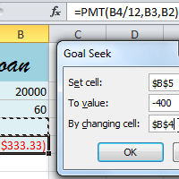
Let's saying you're trying to solve a complicated problem with Excel, like calculating an unknown value. You could try solving it on your own, plugging in different numbers until you find the right answer. However, this method could take a lot of time and effort.
Instead of calculating the answer by yourself, you could use a powerful Excel tool called what-if analysis. This feature makes it easier to experiment with your data. In this lesson, we'll show you how to use what-if analysis to answer different types of questions.
Excel includes many powerful tools to perform complex mathematical calculations, including what-if analysis. This feature can help you experiment and answer questions with your data, even when the data is incomplete. In this lesson, you'll learn how to use a what-if analysis tool called Goal Seek.
Optional: You can download this example for extra practice.
When you create a formula or function in Excel, you put various parts together to calculate a result. Goal Seek works in the opposite way: It lets you start with the desired result, and it calculates the input value that will give you that result. We'll use a few examples to show how to use Goal Seek.
Let's say you're enrolled in a class. You currently have a grade of 65, and you need at least a 70 to pass the class. Luckily, you have one final assignment that might be able to raise your average. You can use Goal Seek to find out what grade you need on the final assignment to pass the class.
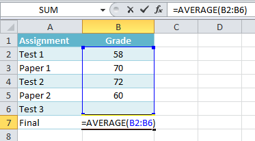
In the image below, you can see that the grades on the first four assignments are 58, 70, 72, and 60. Even though we don't know what the fifth grade will be, we can go ahead and write a formula or function that calculates the final grade. In this case, each assignment is weighted equally, so all we have to do is average all five grades by typing =AVERAGE(B2:B6). Once we use Goal Seek, cell B6 will show us the minimum grade we'll need to make on the final assignment.
 Function calculating the monthly payment
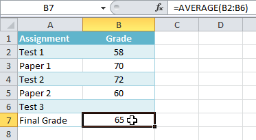 Selecting cell B7
 Selecting Goal Seek from the drop-down menu
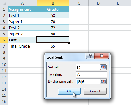 Entering the desired values into the dialog box and clicking OK
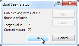 Clicking OK
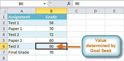 The completed Goal Seek and calculated value
Let's say you need a loan to buy a new car. You already know you want a loan amount of $20,000, a 60-month term—the length of time it takes to pay off the loan—and a payment of no more than $400 per month. However, you're not sure yet what the interest rate will be.
In the image below, you can see that Interest Rate is left blank and Payment is $333.33. This is because the payment is being calculated by a specialized function called the PMT (Payment) function, and $333.33 is what the monthly payment would be if there were no interest ($20,000 divided by 60 monthly payments).
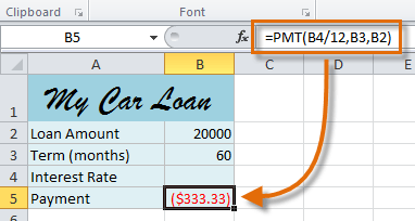 Function calculating the monthly payment
If we typed different values into the empty Interest Rate cell, we could eventually find the value that causes Payment to be $400, and that would be the highest interest rate that we could afford. However, Goal Seek can do this automatically by starting with the result and working backward.
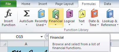 The Financial command
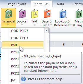 Selecting the PMT function
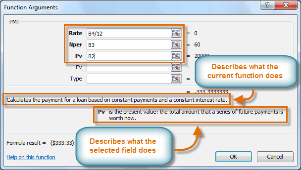 Entering values into the necessary fields
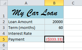 The monthly payment, not including interest
Now that we've added the PMT function, we can use Goal Seek to find the interest rate we'll need.
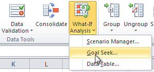 Selecting Goal Seek
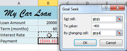 Entering values into the Goal Seek fields
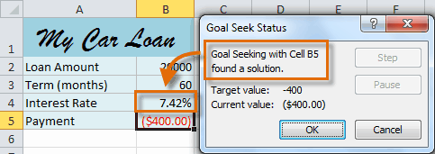 Solution found by Goal Seek
For more advanced projects, you may want to consider the other types of what-if analysis: scenarios and data tables. Rather than start from the desired result and working backward like with Goal Seek, you can use these options to test multiple values and see how the results change.
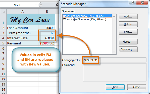 Using the Scenario Manager to compare different options
For more information on scenarios, check out this article from Microsoft.
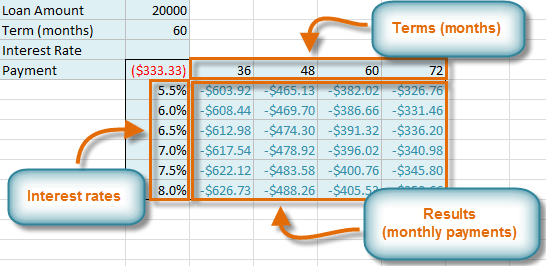 Data tables
For more information on data tables, check out this article from Microsoft.
/en/excel2010/merging-copies-of-a-shared-workbook/content/