Google Sheets: Formatting Cells

Lesson 10: Formatting Cells

/en/googlespreadsheets/modifying-columns-rows-and-cells/content/

Introduction

After you've added a lot of content to a spreadsheet, it can sometimes be difficult to view and read all of your information easily. Formatting allows you to customize the look and feel of your spreadsheet, making it easier to view and understand.

In this lesson, you'll learn how to modify the size, style, and color of text in your cells. You will also learn how to set text alignment and add borders and background colors to your cells.

Formatting cells

Every cell in a new spreadsheet uses the same default formatting. As you begin to build a spreadsheet, you can customize the formatting to make your information easier to view and understand. In our example, we will be using a spreadsheet to plan and organize a garden plot.

Watch the video below to learn the basics of formatting cells.

To change the font size:

Modifying the font size can help call attention to important cells and make them easier to read. In our example, we will be increasing the size of our header cells to help distinguish them from the rest of the spreadsheet.

  1. Select the cell or cells you want to modify.
    Selecting the desired cells
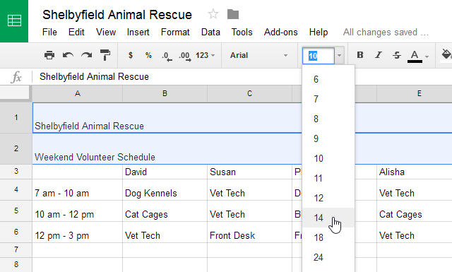
  2. Locate and select the Font Size button in the toolbar, then choose the desired font size from the drop-down menu. In our example, we will choose 14 to make the text larger.
    Changing the font size
  3. The text will change to the new font size.
    The updated font size

To change the font:

Choosing a different font can help to further separate certain parts of your spreadsheet—like the header cells—from the rest of your information.

  1. Select the cell or cells you want to modify.
  2. Locate and select Format in the toolbar menu.
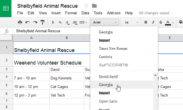
  3. Hover the mouse over Font, then select a new font from the drop-down menu. In our example, we'll select Georgia.
    Changing the font style
  4. The text will change to the new font.
    The new font style

To change the text color:

  1. Select the cell or cells you want to modify.
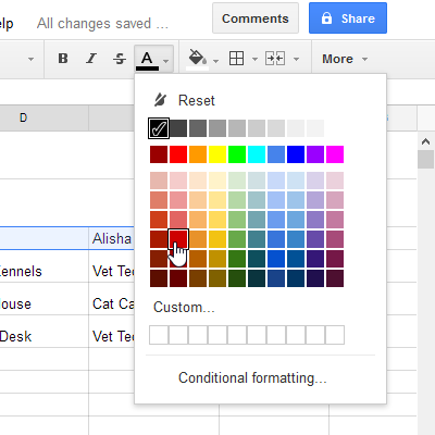
  2. Locate and select the Text color button in the toolbar.
    Changing the text color
  3. A drop-down menu of different text colors will appear.
  4. Select the color you want to use. In our example, we'll select red.
    Choosing a text color
  5. The text will change to the new color.
    The new text color

To make text bold:

  1. Select the text you want to modify.
  2. To bold text, click the Bold text button or press Ctrl+B (Windows) or Command+B (Mac) on your keyboard.
    Bolding text
  3. The text will change to bold.
    The bolded text

Press Ctrl+I (Windows) or Command+I (Mac) on your keyboard to add italics. Press Ctrl+U (Windows) or Command+U (Mac) to add underlining.

Italics and underlining

Text alignment

By default, any text entered into your spreadsheet will be aligned to the bottom-left of a cell. Any numbers will be aligned to the bottom-right of a cell. Changing the alignment of your cell content allows you to choose where the content will appear.

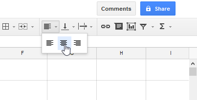
To modify the horizontal text alignment:

  1. Select the text you want to modify.
    Clicking the Align button
  2. Click the Horizontal align button in the toolbar, then select the desired alignment from the drop-down menu.
    Choosing the horizontal alignment
  3. The text will realign.
    The new horizontal alignment

To modify the vertical text alignment:

  1. Select the text you want to modify.
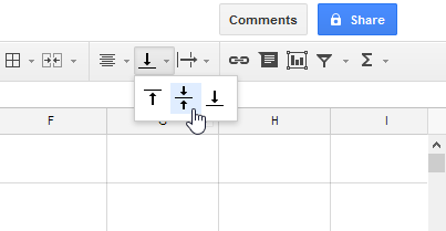
  2. Click the Vertical align button in the toolbar, then choose the desired alignment from the drop-down menu.
    Choosing the vertical alignment
  3. The text will realign.
    The new vertical alignment

You can apply both vertical and horizontal alignment settings to any cell.

Cell borders and background colors

Cell borders and background colors make it easy to create clear and defined boundaries for different sections of your spreadsheet.

To add cell borders:

  1. Select the cell or cells you want to modify.
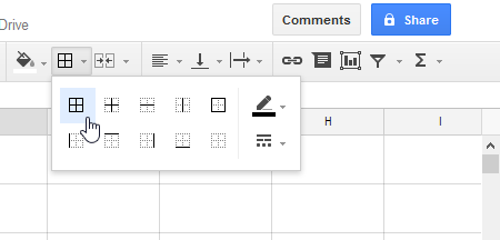
    Clicking the Borders button
  2. Select the Borders button and choose the desired border option from the drop-down menu. In our example, we'll choose to display all cell borders.
    Selecting the cell border settings
  3. The new cell borders will appear.
    The new cell borders

To change the fill color:

It's easy to change the background color of any cell, which is known as the fill color.

  1. Select the cell or cells you want to modify.
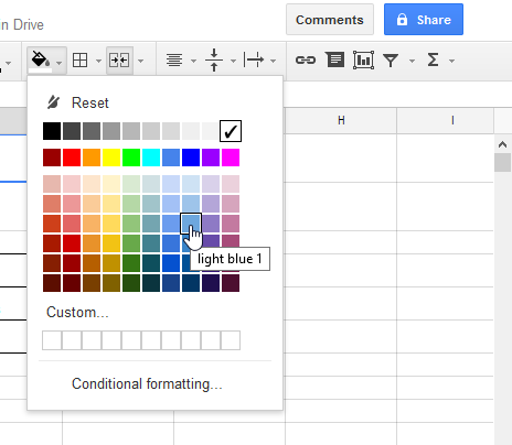
  2. Locate and select the Fill color button from the toolbar.
    Changing the text background color
  3. Select a color from the drop-down menu. In our example, we'll choose blue.
    Choosing a text background color
  4. The new fill color will appear.
    The new text background color

Formatting text and numbers

The ability to apply specific formatting for text and numbers is one of the most powerful tools in Google Sheets. Instead of displaying all cell content in exactly the same way, you can use formatting to change the appearance of dates, times, decimals, percentages (%), currency ($), and much more.

Learn more about formatting numbers in our Understanding Number Formats lesson.

Challenge!

  1. Open our example spreadsheet. Make sure you're signed in to Google, then click File > Make a copy.
  2. Select cells A1:E6. Change the horizontal alignment to center and the vertical alignment to middle.
  3. Select cells B3:E3. Bold the text and add an outside border.
  4. Select the merged cell in row 1 and change the font to something other than Arial.
  5. With the cell still selected, change the font size to 18 pt and bold the text.
  6. For the same cell, change the fill color to purple and the font color to white.
  7. When you're finished, your spreadsheet should look something like this:
    formatting cells challenge example

/en/googlespreadsheets/working-with-multiple-sheets/content/